Simulation based calibration

This example demonstrates how to use the SBC class for simulation-based calibration, supporting both PyMC and Bambi models.

from arviz_plots import plot_ecdf_pit, style
import numpy as np
import simuk
style.use("arviz-variat")

PyMC

First, define a PyMC model. In this example, we will use the centered eight schools model.

import pymc as pm

data = np.array([28.0, 8.0, -3.0, 7.0, -1.0, 1.0, 18.0, 12.0])
sigma = np.array([15.0, 10.0, 16.0, 11.0, 9.0, 11.0, 10.0, 18.0])

with pm.Model() as centered_eight:
    mu = pm.Normal('mu', mu=0, sigma=5)
    tau = pm.HalfCauchy('tau', beta=5)
    theta = pm.Normal('theta', mu=mu, sigma=tau, shape=8)
    y_obs = pm.Normal('y', mu=theta, sigma=sigma, observed=data)

Pass the model to the SBC class, set the number of simulations to 100, and run the simulations. This process may take some time since the model runs multiple times (100 in this example).

sbc = simuk.SBC(centered_eight,
    num_simulations=100,
    sample_kwargs={'draws': 25, 'tune': 50})

sbc.run_simulations();

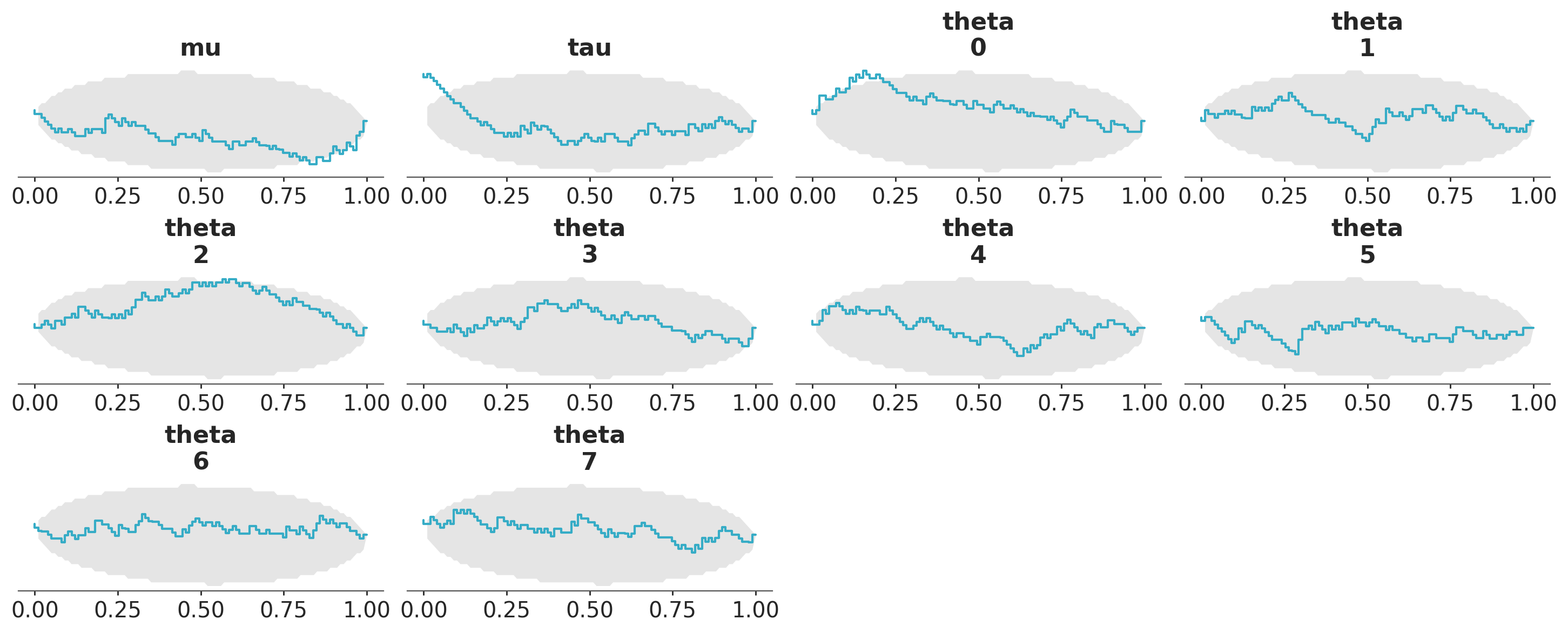
To compare the prior and posterior distributions, we will plot the results from the simulations, using the ArviZ function plot_ecdf_pit. We expect a uniform distribution, the gray envelope corresponds to the 94% credible interval.

plot_ecdf_pit(sbc.simulations,
              pc_kwargs={'col_wrap':4},
              plot_kwargs={"xlabel":False},
)

<arviz_plots.plot_collection.PlotCollection at 0x7bae5ede1650>

Bambi

Now, we define a Bambi Model.

import bambi as bmb
import pandas as pd

x = np.random.normal(0, 1, 200)
y = 2 + np.random.normal(x, 1)
df = pd.DataFrame({"x": x, "y": y})
bmb_model = bmb.Model("y ~ x", df)

Pass the model to the SBC class, set the number of simulations to 100, and run the simulations. This process may take some time, as the model runs multiple times

sbc = simuk.SBC(bmb_model,
    num_simulations=100,
    sample_kwargs={'draws': 25, 'tune': 50})

sbc.run_simulations();

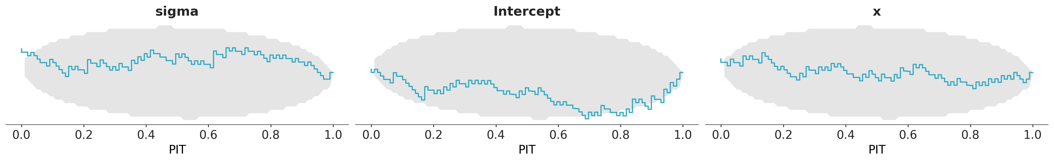
To compare the prior and posterior distributions, we will plot the results from the simulations. We expect a uniform distribution, the gray envelope corresponds to the 94% credible interval.

plot_ecdf_pit(sbc.simulations)

<arviz_plots.plot_collection.PlotCollection at 0x7bae605ab010>

Numpyro

We define a Numpyro Model, we use the centered eight schools model.

import numpyro
import numpyro.distributions as dist
from jax import random
from numpyro.infer import NUTS
y = np.array([28.0, 8.0, -3.0, 7.0, -1.0, 1.0, 18.0, 12.0])
sigma = np.array([15.0, 10.0, 16.0, 11.0, 9.0, 11.0, 10.0, 18.0])
def eight_schools_cauchy_prior(J, sigma, y=None):
    mu = numpyro.sample("mu", dist.Normal(0, 5))
    tau = numpyro.sample("tau", dist.HalfCauchy(5))
    with numpyro.plate("J", J):
        theta = numpyro.sample("theta", dist.Normal(mu, tau))
    numpyro.sample("y", dist.Normal(theta, sigma), obs=y)
# We use the NUTS sampler
nuts_kernel = NUTS(eight_schools_cauchy_prior)

Pass the model to the SBC class, set the number of simulations to 100, and run the simulations. For numpyro model, we pass in the data_dir parameter.

sbc = simuk.SBC(nuts_kernel,
    sample_kwargs={"num_warmup": 50, "num_samples": 75},
    num_simulations=100,
    data_dir={"J": 8, "sigma": sigma, "y": y},
)
sbc.run_simulations()

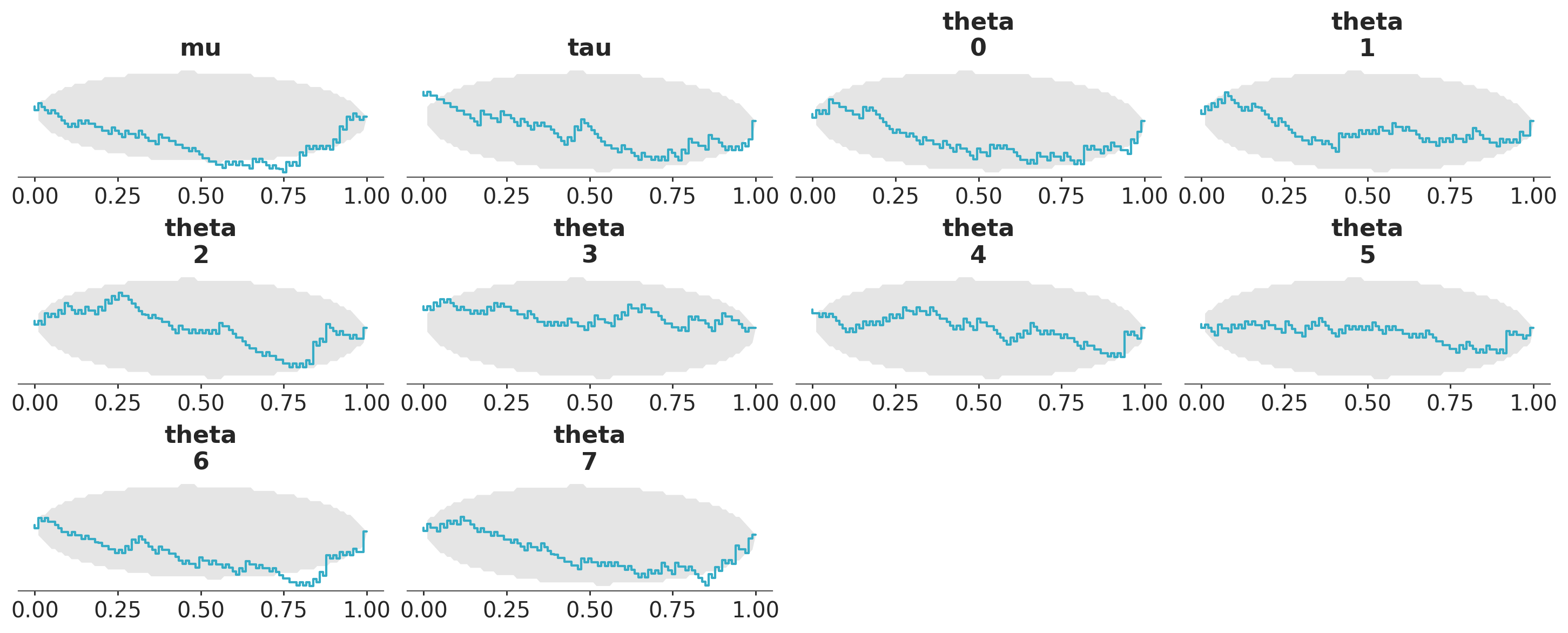
To compare the prior and posterior distributions, we will plot the results. We expect a uniform distribution, the gray envelope corresponds to the 94% credible interval.

plot_ecdf_pit(sbc.simulations, 
              pc_kwargs={'col_wrap':4},
              plot_kwargs={"xlabel":False}
)

<arviz_plots.plot_collection.PlotCollection at 0x7bae34d0ba50>